Color Cell Background Partially in Excel using Data Bars

For Microsoft Excel 2016 users it is only a few clicks to color cell backgrounds partially forming a horizantal bar chart according to the numeric values that cell has for defining the colored percentage of the cell. In Microsoft Excel 2016, users can use the feature Conditional Formatting with Data Bars tool to color only a portion of the cell background dynamically.

I recently required to display the values stored in an Excel sheet column visually. The best way was to color the background of cells partially as a percentage of the whole cell. So I simply chosed to use the Data Bars Conditional Formatting tool for coloring Excel sheet cells as shown in this tutorial.

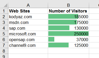
Here is an example case in Excel 2016 document in which the background of the column cells are highlighted with green, choosen color. The Excell cell with the biggest value is colored full in its background. Other cell backgrounds are partly colored forming a horizontal bar shape according to their value percentage when compared to the highest value.

Launch Microsoft Office 2016 Excel application.
Open your Excel document.
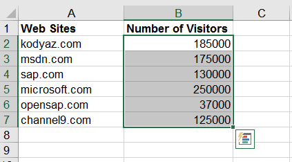
Highlight or select the data cells in the column

Using Excel 2016 ribbon menu, from Home tab, click Conditional Formatting icon under Styles section.

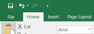
Home tab

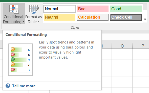
Styles > Conditional Formatting

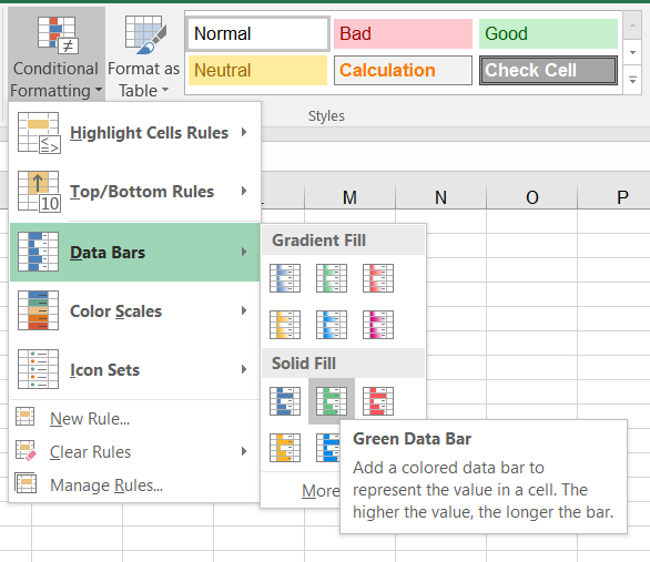
As seen in above screenshot, Conditional Formatting provides Data Bars tools which are ready to apply on selected cells.

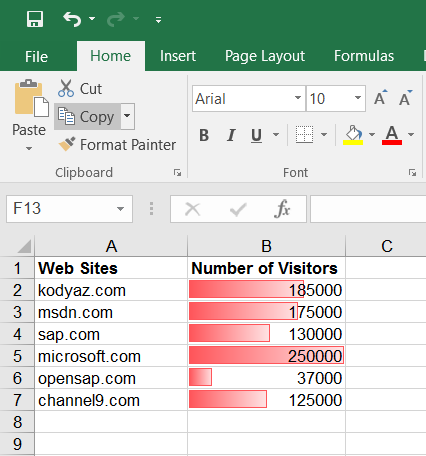
If you want a more fancy representation on your Excel document, you can choose Gradient Fill and select a color for cell backgrounds among different options. Or you can simply continue bar selecting a color from Solid Fill part.

Here is an other representation of the same values in the Excel 2016 Office document using gradient fill using red color as data bars coloring as cell backgrounds accoring to cell values.